As a data scientist working with biological data, the programming language I use on a daily basis is Python. However, I sometimes find myself needing to use an R package, such as those provided by Bioconductor. For me this is most often the excellent MSstats R package from Meena Choi (@MeenaChoi) and folks in Olga Vitek’s lab (@olgavitek). Although it has always been possible to write R scripts alongside my Python scripts and Jupyter notebooks, I find it cumbersome to switch back and forth between them, particularly when it involves generating unnecessary intermediate files.
In this post I’ll show you how I use the MSstats R package from within a Python script or Jupyter notebook, providing an example for how you can use the occasional R package in your own analyses. This post will assume that you’re comfortable programming in Python and that you’re familiar with the Pandas, NumPy, and Matplotlib Python packages.1 Additionally, I’ll assume that you have some familiarity with R programming, since you’re reading this post. I’ll be using proteomics data as an example, but understanding it is not critical for learning from this post.
This entire post is available as a Jupyter notebook on GitHub: https://github.com/wfondrie/msstats-demo
Setup
If you want to follow along with this post, you’ll need to install a few things. I use conda as my package manager for Python and R whenever possible.2 First, we’ll create a new conda environment, msstats-demo, and install the necessary packages from the bioconda and conda-forge channels. I’ve created a conda environment YAML file that looks like this:
# https://github.com/wfondrie/msstats-demo/environment.yaml
name: msstats-demo
channels:
  - bioconda
  - conda-forge
  - defaults
dependencies:
  - ppx>=1.2.5                   # For downloading data
  - bioconductor-msstats==4.2.0  # The MSstats R package
  - notebook                     # Jupyter notebook
  - ipywidgets                   # For progress bars
  - pandas                       # DataFrames for tabular data
  - numpy                        # To do math
  - matplotlib                   # The de facto standard Python plotting library
  - seaborn                      # Make matplotlib plots pretty
  - rpy2                         # For using R packages in Python!
Let’s start by creating the conda environment from this file:
conda env create -f https://raw.githubusercontent.com/wfondrie/msstats-demo/main/environment.yaml
Then activate our new conda environment:
conda activate msstats-demo
Now let’s fire up Python. If you want to use a Jupyter notebook, you can launch it with:
jupyter notebook
Then click New → Python 3 (ipykernel) to open a new notebook.
Getting started
For this post, we’re going to reproduce an analysis of the the dataset from Selevsek et al as performed in the MassIVE.quant paper. We’ll use Python to download and read the data, process that data with the MSstats R package, then recreate the volcano plot in Figure 2j with Python. Let’s start by loading the libraries we’ll need into our Python session:
import ppx
import numpy as np
import pandas as pd
import matplotlib.pyplot as plt
import seaborn as sns

# These will let us use R packages:
from rpy2.robjects.packages import importr
from rpy2.robjects import pandas2ri

# Convert pandas.DataFrames to R dataframes automatically.
pandas2ri.activate()
The rpy2 Python package will perform the magic that allows us to use R packages in our Python session. The importr function give us the power to import R packages and pandas2ri—along with the subsequent pandas2ri.activate() line—will allow our Pandas DataFrames to be automically converted into R data frames when used as input to an R function.
We also need to set up a plotting style that looks nice on my website:
# Set plotting theme:
primary = "#404040"
accent = "#24B8A0"
pal = sns.color_palette([primary, accent])
style = {
    "axes.edgecolor": primary,
    "axes.labelcolor": primary,
    "text.color": primary,
    "xtick.color": primary,
    "ytick.color": primary,
}

sns.set_palette(pal)
sns.set_context("talk")
sns.set_style("ticks", style)
Now let’s download the dataset from the MassIVE mass spectrometry data repository under the accession RMSV000000251. We’ll use the ppx Python package to do this:
proj = ppx.find_project("RMSV000000251")

# The proteomics data:
quant_file = "2019-06-03_mnchoi_bb4aeafb/quant/Selevsek2015-MSstats-input-90nodup-i.csv"

# The annotation file:
annot_file = "2019-06-03_mnchoi_bb4aeafb/metadata/Selevsek2015_DIA_Skyline_all_annotation.csv"

# The local paths to them:
quant_path, annot_path = proj.download([quant_file, annot_file], silent=True)
We can then read the proteomics data into our Python session using Pandas:
quant_df = pd.read_csv(quant_path, dtype={"StandardType": str})
quant_df.head() # View the first five rows
| ProteinName | PeptideSequence | PeptideModifiedSequence | PrecursorCharge | PrecursorMz | FragmentIon | ProductCharge | ProductMz | IsotopeLabelType | Condition | BioReplicate | FileName | Area | StandardType | Truncated | DetectionQValue | |
|---|---|---|---|---|---|---|---|---|---|---|---|---|---|---|---|---|
| 0 | Biognosys standards | LGGNEQVTR | LGGNEQVTR | 2 | 487.256705 | y7 | 1 | 803.400606 | light | NaN | NaN | nselevse_L120412_001_SW.wiff | 353982.43750 | iRT | False | NaN |
| 1 | Biognosys standards | LGGNEQVTR | LGGNEQVTR | 2 | 487.256705 | y7 | 1 | 803.400606 | light | NaN | NaN | nselevse_L120412_002_SW.wiff | 408376.46875 | iRT | False | NaN |
| 2 | Biognosys standards | LGGNEQVTR | LGGNEQVTR | 2 | 487.256705 | y7 | 1 | 803.400606 | light | NaN | NaN | nselevse_L120412_003_SW.wiff | 437152.65625 | iRT | False | NaN |
| 3 | Biognosys standards | LGGNEQVTR | LGGNEQVTR | 2 | 487.256705 | y7 | 1 | 803.400606 | light | NaN | NaN | nselevse_L120412_004_SW.wiff | 344150.12500 | iRT | False | NaN |
| 4 | Biognosys standards | LGGNEQVTR | LGGNEQVTR | 2 | 487.256705 | y7 | 1 | 803.400606 | light | NaN | NaN | nselevse_L120412_005_SW.wiff | 383755.62500 | iRT | False | NaN |
We also need to read the annotation data using Pandas:
annot_df = pd.read_csv(annot_path)
annot_df.head()
| Condition | BioReplicate | Run | |
|---|---|---|---|
| 0 | T000 | 1 | nselevse_L120412_001_SW.wiff |
| 1 | T000 | 2 | nselevse_L120412_002_SW.wiff |
| 2 | T000 | 3 | nselevse_L120412_003_SW.wiff |
| 3 | T015 | 1 | nselevse_L120412_004_SW.wiff |
| 4 | T015 | 2 | nselevse_L120412_005_SW.wiff |
Finally, we need to create a contrast matrix that will define the comparisons we want to test with MSstats:
cols = annot_df["Condition"].unique()
cols.sort()

rows = ["T1-T0", "T2-T0", "T3-T0", "T4-T0", "T5-T0"]

contrasts = [
    [-1, 1, 0, 0, 0, 0],
    [-1, 0, 1, 0, 0, 0],
    [-1, 0, 0, 1, 0, 0],
    [-1, 0, 0, 0, 1, 0],
    [-1, 0, 0, 0, 0, 1],
]

contrast_df = pd.DataFrame(
    contrasts,
    columns=cols,
    index=rows,
)

contrast_df
| T000 | T015 | T030 | T060 | T090 | T120 | |
|---|---|---|---|---|---|---|
| T1-T0 | -1 | 1 | 0 | 0 | 0 | 0 |
| T2-T0 | -1 | 0 | 1 | 0 | 0 | 0 |
| T3-T0 | -1 | 0 | 0 | 1 | 0 | 0 |
| T4-T0 | -1 | 0 | 0 | 0 | 1 | 0 |
| T5-T0 | -1 | 0 | 0 | 0 | 0 | 1 |
Run MSstats in Python using rpy2
Now for the fun part: let’s run MSstats without leaving our Python session. Just like if we were using R directly, we first need to import the libraries that we’ll be using. This looks a little different using rpy2, but ultimately we assign the imported R package to a variable that we can use like any other Python package. Here, we import MSstats:
MSstats = importr("MSstats")
Next, we’ll perform our MSstats data processing. Note that each of these functions actually call the underlying MSstats R package. The rpy2 Python package does all of the work tranforming our Pandas DataFrames (quant_df, annot_df, and contrast_df) into R data frames that MSstats can use. When each function is complete, it returns an R object. Fortunately, we’ve setup rpy2 to automatically convert R data frames back into Pandas DataFrames, allowing us to use the results seamlessly. The final output returned by MSstats in this analysis (results below) will be a Pandas DataFrame containing the p-values for each protein for contrasts that we specified in our contrast matrix (contrast_df).
If you’re following along, this next step may take a few minutes. Go ahead and enjoy a cup of coffee or your favorite beverage while it’s running.
raw = MSstats.SkylinetoMSstatsFormat(
    quant_df,
    annotation=annot_df,
    removeProtein_with1Feature=True,
    use_log_file=False,
)

processed = MSstats.dataProcess(
    raw,
    use_log_file=False,
)

# Note that the 'contrast_matrix' argument below
# is actually 'contrast.matrix' in the MSstats
# R package. rpy2 swaps '.' for '_' so that it
# becomes a valid Python variable name.
results, *_ = MSstats.groupComparison(
    contrast_matrix=contrast_df,
    data=processed,
    use_log_file=False,
)
INFO  [2022-01-07 15:30:17] ** Raw data from Skyline imported successfully.
INFO  [2022-01-07 15:31:07] ** Raw data from Skyline cleaned successfully.
INFO  [2022-01-07 15:31:07] ** Using provided annotation.
INFO  [2022-01-07 15:31:07] ** Run labels were standardized to remove symbols such as '.' or '%'.
INFO  [2022-01-07 15:31:07] ** The following options are used:
  - Features will be defined by the columns: IsotopeLabelType, PeptideSequence, PrecursorCharge, FragmentIon, ProductCharge
  - Shared peptides will be removed.
  - Proteins with a single feature will be removed.
  - Features with less than 3 measurements across runs will be removed.
INFO  [2022-01-07 15:31:07] ** Rows with values of StandardType equal to iRT are removed
INFO  [2022-01-07 15:31:08] ** Intensities with values of Truncated equal to TRUE are replaced with NA
INFO  [2022-01-07 15:31:11] ** Intensities with values smaller than 0.01 in DetectionQValue are replaced with 0
INFO  [2022-01-07 15:31:11] ** Sequences containing DECOY, Decoys are removed.
INFO  [2022-01-07 15:31:16] ** Features with all missing measurements across runs are removed.
INFO  [2022-01-07 15:31:19] ** Shared peptides are removed.
INFO  [2022-01-07 15:31:28] ** Multiple measurements in a feature and a run are summarized by summaryforMultipleRows: sum
INFO  [2022-01-07 15:31:28] ** Features with one or two measurements across runs are removed.
INFO  [2022-01-07 15:31:30] Proteins with a single feature are removed.
INFO  [2022-01-07 15:31:34] ** Run annotation merged with quantification data.
INFO  [2022-01-07 15:31:35] ** Features with one or two measurements across runs are removed.
INFO  [2022-01-07 15:31:36] ** Fractionation handled.
INFO  [2022-01-07 15:31:39] ** Updated quantification data to make balanced design. Missing values are marked by NA
INFO  [2022-01-07 15:31:40] ** Finished preprocessing. The dataset is ready to be processed by the dataProcess function.
INFO  [2022-01-07 15:31:44] ** There are 499195 intensities which are zero or less than 1. These intensities are replaced with 1
INFO  [2022-01-07 15:31:47] ** Log2 intensities under cutoff = 7.4056  were considered as censored missing values.
INFO  [2022-01-07 15:31:47] ** Log2 intensities = NA were considered as censored missing values.
INFO  [2022-01-07 15:31:48] ** Use all features that the dataset originally has.
INFO  [2022-01-07 15:31:48]
 # proteins: 2189
 # peptides per protein: 1-157
 # features per peptide: 1-6
INFO  [2022-01-07 15:31:48]
                    T000 T015 T030 T060 T090 T120
             # runs    3    3    3    3    3    3
    # bioreplicates    3    3    3    3    3    3
 # tech. replicates    1    1    1    1    1    1
INFO  [2022-01-07 15:31:50] Some features are completely missing in at least one condition:
 KEGLDGHR_2_y3_1,
 KEGLDGHR_2_y4_1,
 KEGLDGHR_2_y5_1,
 KEGLDGHR_2_y7_1,
 VQHPNIVNLLDSFVEPISK_3_b8_1 ...
INFO  [2022-01-07 15:31:50]  == Start the summarization per subplot...
  |======================================================================| 100%
INFO  [2022-01-07 15:58:26]  == Summarization is done.
INFO  [2022-01-07 15:58:34]  == Start to test and get inference in whole plot ...
  |======================================================================| 100%
INFO  [2022-01-07 15:59:19]  == Comparisons for all proteins are done.
Now that the process is complete, we can verify that results is a Pandas DataFrame containing our MSstats results:
results.head()
| Protein | Label | log2FC | SE | Tvalue | DF | pvalue | adj.pvalue | issue | MissingPercentage | ImputationPercentage | |
|---|---|---|---|---|---|---|---|---|---|---|---|
| 1 | Q0250 | T1-T0 | 0.001292 | 0.111103 | 0.011625 | 10 | 0.990953 | 0.995633 | None | 0.033333 | 0.033333 |
| 2 | Q0250 | T2-T0 | -0.106017 | 0.111103 | -0.954230 | 10 | 0.362464 | 0.533674 | None | 0.066667 | 0.066667 |
| 3 | Q0250 | T3-T0 | -0.123694 | 0.111103 | -1.113334 | 10 | 0.291610 | 0.442217 | None | 0.100000 | 0.100000 |
| 4 | Q0250 | T4-T0 | 0.267058 | 0.111103 | 2.403706 | 10 | 0.037080 | 0.111271 | None | 0.033333 | 0.033333 |
| 5 | Q0250 | T5-T0 | 0.242798 | 0.111103 | 2.185348 | 10 | 0.053757 | 0.120164 | None | 0.033333 | 0.033333 |
We’ve successfully run MSstats without leaving our Python session!
Reproduce a figure panel from the paper
The only task left is reproduce a panel from a figure in the MassIVE.quant paper. We’ll recreate the volcano plot from Figure 2j and see how close our results are to the original.3 However, we’ll make this plot using seaborn and matplotlib in our Python session!
# Filter the results for the points we want to plot
results = results.loc[results["adj.pvalue"] > 0, :]
results = results.loc[results["Label"] == "T5-T0", :]
results["accepted"] = results["adj.pvalue"] <= 0.05
results["neg_log_pvalue"] = -np.log10(results["adj.pvalue"])

# Get the number of up and down-regulated proteins
n_up = ((results["log2FC"] > 0) & results["accepted"]).sum()
n_down = ((results["log2FC"] < 0) & results["accepted"]).sum()

# Create the figure
plt.figure()

# Create the Scatter plot
sns.scatterplot(
    data=results,
    x="log2FC",
    y="neg_log_pvalue",
    hue="accepted",
    legend=False,
    s=20
)

# Add annotations
plt.text(
    x=0.02,
    y=0.98,
    s=f"Up: {n_up}\nDown: {n_down}",
    transform=plt.gca().transAxes,
    va="top",
)

# Add the horizontal line
plt.axhline(-np.log10(0.05), linestyle="dashed", zorder=0)

# Add labeling
plt.xlabel("log2 fold change")
plt.ylabel("-log10(adjusted p-value)")
plt.title("Skyline:all")

# Set the axes limits
plt.ylim(0, 8)
plt.xlim(-4, 4)

# Show the plot
plt.show()
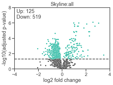
This looks pretty close to the original to me, particularly considering that we didn’t make any attempt to match our software versions with the original analysis. The number of up and down-regulated proteins is nearly identical, with our analysis finding one fewer down-regulated protein than in the original.
Conclusion
The rpy2 Python package provides a pretty convenient way to use the occassional R package in Python, and I’ve shown you how to use it to run MSstats. Finally, I’ll leave you with this: if you want to use the occasional Python package in R, try the reticulate R package.
-
If these are not familiar and you want to learn, I recommend the “Plotting and Programming in Python” Software Carpentry course. ↩︎
-
If you need to install conda, I’d recommend the miniconda distribution. ↩︎
-
I haven’t included the original figure for copyright reasons. ↩︎